Reference
This is the mujpy Reference Manual, v. 2.7.3. Any fit can be lauched also without Jupyterlab by means of the following classes:
musuite
from mujpy.musuite import suite
the_suite = suite(datafile,runlist,grp_calib,offset,startuppath,**kwargs)
where datafile is a string containing the path (see Header), runlist is the list of run numbers in the suite of runs (see suite), grp_calib list of dictionaries (see groups), offset is a string containing an integer (see `offset`_), startuppath is a string containing the path where the log folders (named fit, csv, cache) will be written. This class performs the functions roughly described in suite
mufit
from mujpy.mufit import mufit
the_fit = mufit(suite,dashboard,**kwargs)
where suite is an instantiation of suite, e.g. the_suite in musuite, dashboard is a string containing the full path to a dashbord json file (see Dashboard json, and kwargs are
- chain = False, chain = True to use parameter values from previous run as guess for next
- dash = None, internal parameter, used by mudash to direct log output
- initialize_only = False, if mufit is used just to load parameters for a guess plot
- grad = False, if True and the fit is global then gradients of the chi_square function are computed analytically. This option is not recommended, convergence is 1.5 times slower and it requires much closer guess to the minimum
- scan = None, tells mufit to order csv file in increasing order of run number, scan = ‘T’ increasing temperatures, ‘B’ increasing fields.
This class performs a single fit, a sequential multigroup or suite fit, a global multigroup or a global suite fit (see fit).
A global fit minimizes a single chi square, that is the sum of the chi squares of all data sets. The class automatically identifies the type of fit on the basis of the dashboard json file:
- A1, single run, single group fit; switches automatically to calibration mode if the first component is ‘al’
- A20, single run, sequential multi group fit; switches automatically to calibration mode if the first component is ‘al’
- A21, single run, global multi group fit; switches automatically to calibration mode if the first component is ‘al’
- B1, sequential multirun, single group fit
- B20, sequential multirun, sequential multigroup fit
- B21, sequential multirun, global multigroup fit
- C1, multirun single group global fit
Dashboard json
This json file contains the full description of any legal fit model. See templates for examples. The file name starts with the model name (see fit_model) and its file spec is .json. It resembles a python dictionary, containing the following items:
- “version”: “a string”, see fit_model
- “fit_range”: “0,20000,4”, see fit_model
- “offset”: 20, see fit_model
- “userpardicts_guess”: [], see fit dashboard
- “model_guess: [], see fit dashboard
Experienced users can write the json file from scratch and run the fits with few command line instructions, but this mode is error prone. Jupyterlab contains a json editor that facilitates the task. However, the mudash gui interface is provided to make this process more user friendly.
mufitplot
from mujpy.muplotfit import muplotfit
the_plot = muplotfit(plot_range,the_fit,**kwargs)
where plot_range obeys the rules described in `fit'_, the_fit is an instance of mufit, e.g. the_fit as in `mufit`_, and kwardgs are
- guess = False, if True plot the guess parameter values
- rotating_frame_frequencyMHz = 0.0, to plot data in the rotating frame
- fft_range = None, to pass the frequency range for the FFT plot
- real=True, to produce an amplitude FFT plot
- fig_fit=None, to pass the handle of an existing fit figure
- fig_fft=None, to pass the handle of an existing FFT figure
This class produces the (animation) plots
mudash
This class produces the gui interface to mujpy. It is invoked from a jupyter notebook (just start one of the MuDash.ipynb templates).
Here you find a not-so-quick reference for its widgets. Almost each of them has a tiptool: additional instructions appear when hovering with the mouse over the descriptive text or the button.
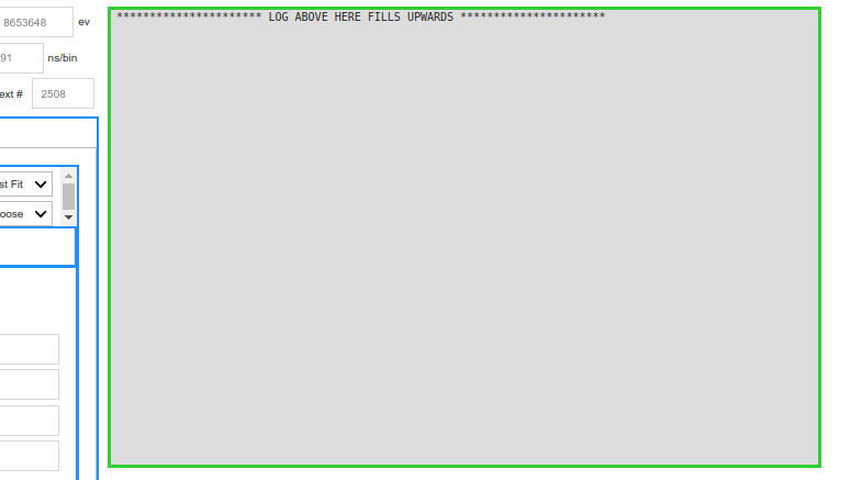
Output
An output area is provided to the left of the gui: the live log from mudash goes there and it is added at the top while the text scrolls down.
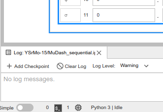
Errors (bugs?) should be intercepted and redirected to the Jupyter Log Console, which can be opened selecting View/Show Log Console in the top Jupiter tabs
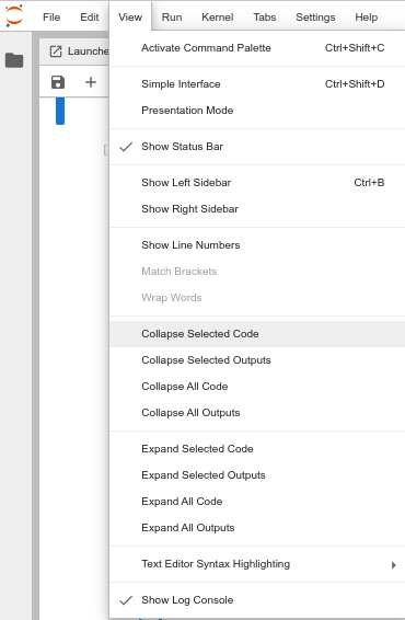
The Jupyter Log Console appears at the bottom
Header
The top part of the mujpy gui contains a logo together with the information on the loaded run (in single run mode) or the loaded master run (in the suite mode the master run is simply that whichi provides mujpy with the data path).
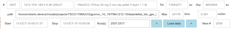
The first line contains the run number, the run title, the total counts, the total counts over the selected grouping of detectors. These are just displays.
The second line contains the path to the data file, which is a template for a suite of runs to be analysed in series. This is an editable Text: modify the path and hit Enter to load a new master data file. Max bins per detector and time resolution are Text displays.
The third line contains start and stop time information, plus
- Run [run suite], a Text input for a list of comma separated run numbers. See suite below for its shorthand notation.
Three last buttons load the previous [master] run, open a file selection gui in the same path, and load the next [master] run, respectively.
single run mode
Individual data set are fitted to models.
suite mode
Individual data set belonging to the loaded run suite are fitted to the model (defined in fit) either in sequence, or in a global fit.
suite
- The musuite class is invoked to:
- load the runs;
- compute the asymmetries for the specified groups for all runs;
- generate a time array with \(t_0=0\), obtained automatically upon loading by the fit described in the setup section;
- more complex syntax allows storing suites of runs, with combination of ,:+ (only one : allowed)
432,433loads the suite of runs 432, 43432:434loads the suite of runs 432, 433, 434432,433, 435:437loads the suite of runs 432, 433, 435, 436, 437432+433loads the sum of these two runs as a single run, etc.
setup
The setup fit identifies the \(t_0=0\) bin according to the data provenance.
PSI data fit the prompt peak of beam positrons that bypass the veto logic. The iminuit fit, minimizing the \(\chi^2\) of the initial data slice and the best fit class muprompt, where
- prepeak and postpeak are the peak interval span (the number of bins) respectively before and after the maximum;
ISIS data fit the buildup of muon counts in the detectors of the pulsed instrument to the best fit class muedge (the integral of the convolution of the beam profile with the pion decay curve, calculated by Mathematica and checkd against data) where
- \(D,N\) and \(t_{00}\) are the fitting parameters, the width of the ISIS pulse, the count rate normalizer and the \(t=0\) position in the raw time array, respectively; in the edge function time \(t_0 = - t_{00}+0.82\tau_\pi\) is used.
- \(\tau_\mu\) and :math:tau_pi are the muon and pion mean lifetimes.
muprompt
muedge
The lower part of the gui is divided in tabs: fit (the main functions), groups (to change detector grouping), about.
fit_model
We describe a single run, single group fit, for simplicity (the same applies to any sequential fit).
A model is composed of predefined additive components, identified by a two-character code (see Component list) and the model naming scheme is based on this code.
A model made of, say, 3 components, ab, ab and de will be called ababde.
The model name is added to the Fit tab label (here it is mgmgmg).
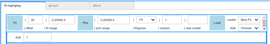
The top fit header contains
- The Fit button launches the iminuit migrad minimization of the model from
- offset, the first good bin, counting from the center prompt peak, over
- the fit range, with a start, stop and a start,stop,pack options, to define the interval and packing for the data minimization (start = k means that the fit starts from bin offset + k). Notice: in this way bins are zero-based (python convention).
- The Plot button produces a plot with either best fit or guess values over
- the plot range with a start, stop and a start,stop,pack options, or a start,stop_early,pack_early,stop_late,pack_late option that produces a double frame window, e.g with small packing at early times and large packing at late times (see also graphic zoom);
- the fit/guess checkbox, to select plot of initial guess or fit result functions.
- version Text (default is ‘1’), is a free tstring to distinguishes fits with the same model and, e.g. different constraints, or different run condtions. It is appended to log file names.
- new model Text area, allows to start an empty new model from scratch: e.g.
mgmgblis a three component model,mg,mg,bl.- The Load fit button opens a GUI file selection of available (past)
jsonfit files, duplicating the Dashboard json file content and adding one or more fit results items at the end. Loading one such file reproduces the input for obtaining again the same fit. Alternatively, empty templates (e.g. more complex global fit ezamples) can be loaded by selecting the following Dropodown- The model Dropdown, selects local best fit or empty templates from the distribution to the mudash gui inteface.
Fit Dashboard
The lower frame contains the fit components selected either by the model syntax or by loding a saved fit.
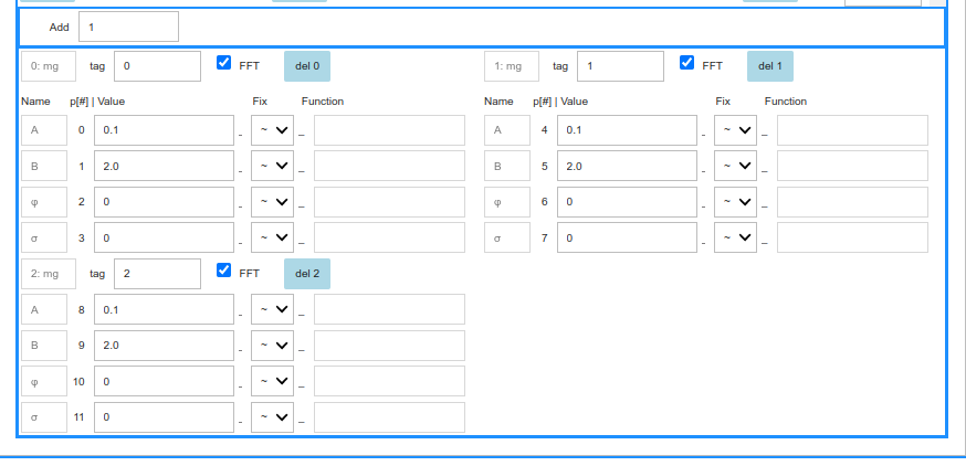
This is a single run or a sequential fit and the top frame contains an Add Integer Text input to add a number of user defined parameters, whose presence tells mudash that the fit will be global. Do not do this initially.
The lower frame is divided in components boxes, in a two-column display.
The first row of each component column starts with a progressively numbered component label (python zero-based), a string tag to disambiguate identical components (e.g. a ‘Fast’ and a ‘SLow’ mg), the FFT checkbox, to include or exclude this component from the model when producing the FFT of the residues, and a button to delete this component from the model.
- The other lines list the component parameters, one row in one column per parameter, each indentified by
- a standard immutable name,
- a dashboard index,
- a Text area for the starting guess value,
- a symbol dropdown:
- ~ free minuit parameter,
- ! fixed parameter
- = the function text area on the right is activated.
- the function Text area, to input symple expressions, such as
p[0], implying that the present parameter and parameter0share the same value. For instance two ml components in model mlml could share their phase parameters. More complex functions may be written, such asp[2]-p[3], orp[0]*exp(p[2]/p[3]), etc. A few constants are defined: \(\pi\), the muon gyromagnetic ratio, \(\gamma_\mu\), the electron gyromagnetic ratio, \(\gamma_e\)
Component list
This is a list of predefined fit components. Adding new ones is straightforward and documentation on how to do this will come.
The two-character codes are supposed to be evocative (?), though ultrashort. E.g. ml is a muon precession with a (partial) asymmetry A, a B local field value (in milliTesla), a phase φ (in degrees) and a Lorentzian relaxation λ (in inverse microseconds); A few constants are defined: \(\pi\), the muon gyromagnetic ratio, \(\gamma_\mu\), the electron gyromagnetic ratio, \(\gamma_e\)
- al, the ratio \(\alpha\) betwen the initial (unpolarized) muon decay count rates, \(N_b\) in Backward counters and \(N_f\) in Forward counters.
- ratio \(\alpha\)
- bl, Lorentz decay:
- asymmetry \(A\)
- Lorentzian rate (\(\mu s^{-1}\)) \(\lambda\)
- bg, Gauss decay:
- asymmetry \(A\)
- Gaussian rate (\(\mu s^{-1}\)) \(\sigma\)
- bs, Stretched exponential decay:
- asymmetry \(A\)
- rate (\(\mu s^{-1}\)) \(\lambda\)
- exponent beta \(\beta\)
- ml, Lorentz decay cosine precession:
- asymmetry \(A\)
- field (mT) \(B\)
- phase (degrees) \(\phi\)
- Loentzian rate (\(\mu s^{-1}\)) \(\lambda\)
- mg, Gauss decay cosine precession:
- asymmetry \(A\)
- field (mT) \(B\)
- phase (degrees) \(\phi\)
- Gaussian rate (\(\mu s^{-1}\)) \(\sigma\)
- ms, Stretched exponential decay cosine precession:
- asymmetry \(A\)
- field (mT) \(B\)
- phase (degrees) \(\phi\)
- rate (\(\mu s^{-1}\)) \(\Lambda\)
- jl, Lorentz decay Bessel precession
- asymmetry \(A\)
- field (mT) \(B\)
- phase (degrees) \(\phi\)
- Lorentzian rate (\(\mu s^{-1}\)) \(\lambda\)
- jg, Gauss decay Bessel precession
- asymmetry \(A\)
- field (mT) \(B\)
- phase (degrees) \(\phi\)
- Gaussian rate (\(\mu s^{-1}\)) \(\sigma\)
- js, Stretched exponential decay Bessel precession:
- asymmetry \(A\)
- field (mT) \(B\)
- phase (degrees) \(\phi\)
- rate (\(\mu s^{-1}\)) \(\Lambda\)
- fm, FMuF coherent evolution:
- asymmetry \(A\)
- dipolar field (mT) \(B_d\)
- Lorentzian rate (\(\mu s^{-1}\)) \(\lambda\)
- kg, Gauss Kubo-Toyabe: static and dynamic, in zero or longitudinal field by G. Allodi Phys Scr 89, 115201
groups
[This tab is not fully implemented and the easiest way to change groups is to duplicate the MuDash notebook and modify by hand the grp_calib list of dictionary in the cell before that invoking mudash]
The groups tab displays and lets the user modify the list of dictionaries that define detector groups.
Warning: counter listing does not follow the zero-based pythonic iterator rule, i.e. the first detector is 1.
Each dictionary represents a single grouping, the ‘Forward’ set of counters, the ‘Backward’ set of counters, plus
about
A few infos and acknowledgements
alpha
the ratio of count rates \(\alpha = N_f/N_b\) between initial (unpolarized) count rates for Backward and Forward grouping.
FFT checkbox
[Sorry, FFT is presently missing in v.2.7.3]
Selects subtracted components for the FFT. E.g. assume best fit model blmgmg with the first two components checked and the last unchecked. The FFT of Residues will show the Fast Fourier Transform of the data minus the model function for the first two components.
Counter inspection
[Sorry, presently missing in v.2.7.3]
- The Counter button produces the plot.
- The next label reminds how many are the available counters.
- The counters Text area allows the selection of the displayed detectors. The syntax is the same as for grouping. It is advisable not to display more than 16 detetcors at a time
- bin, text area to select start, stop, the same range for all chosen detectors. Zoom also by the the graphic zoom
- run dropdown selects one run at a time among the loaded suite.
graphic zoom
All graphic windows display seven icons on the bottom bar
- The
 icon, far right, opens a dialogue for sabìving the plot.
 - The
 icon, next one to the left, corrects the axes position
 - the
 icon, allows zooming in.
 - The first icon on the left,
 , resets the zoom to the orginal ranges
2,3or2:3means that counters 2,3 are grouped together1:5, 10, 15:19means that counters 1,2,3,4,5,10,15,16,17,18,19 are grouped together